Software


Software Architecture#
Micipsa's software stack is organized into a set of layers, each responsible for a distinct concern. Data flows from the sensors at the top, through processing and reasoning layers, down to the actuators at the bottom.
The stack comes in two variants that share nearly all the same layers and topics.
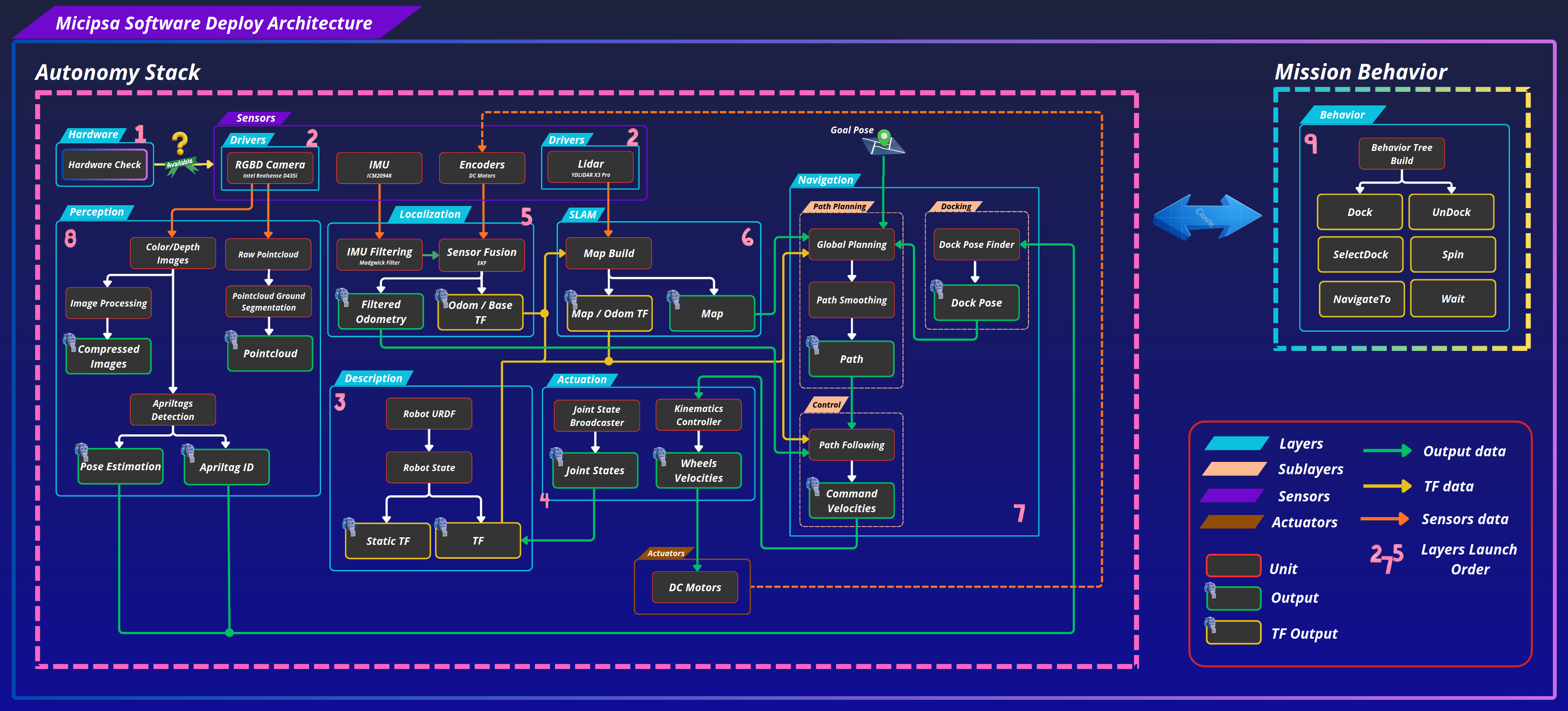
- Deploy: runs on the real robot, with real drivers reading from physical hardware (RGBD camera, IMU, encoders, LiDAR).
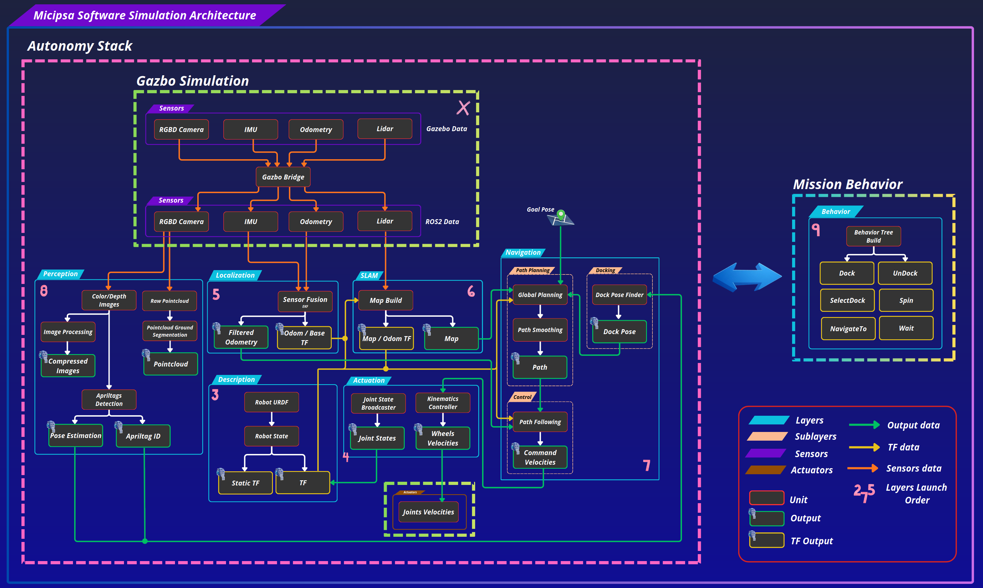
- Simulation: runs in Gazebo with simulated sensors and actuators data.
Deploy#
Simulation#
Micipsa Layers#
Hardware Layer#
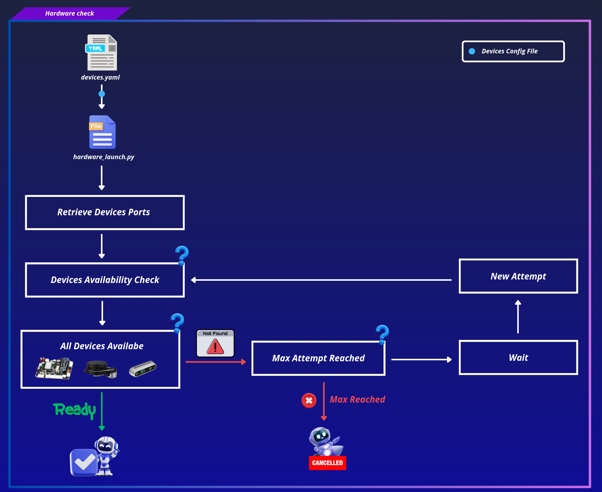
Before any software layer starts, Micipsa performs a hardware check: it verifies that all required hardware is connected and available. If any required hardware is unavailable, the stack will not proceed. This prevents nodes from starting in a broken state where sensors are missing and the robot would behave unpredictably. The hardware layer only exists in the Deploy mode.
Drivers Layer#
The Drivers Layer is responsible for launching and managing the ROS 2 hardware drivers used by the robot:
- RGBD Camera (Intel RealSense D435i) publishes color/depth images and a raw pointcloud
- LiDAR (YDLIDAR X3 Pro) publishes 2D laser scans
The IMU (ICM20948) and Encoders (on the DC motors) are also part of the Sensors sublayer feeding sensor data into Localization, but are read through the hardware component plugin (see Actuation Layer) rather than a standalone driver node.
In simulation, this layer's role is played by the Gazebo Bridge, which republishes Gazebo's simulated RGBD camera, IMU, Odometry, and LiDAR data as the same ROS 2 sensor topics the real drivers would produce so every downstream layer is agnostic to whether it's running on hardware or in sim.
Description Layer#
The description layer is responsible for publishing a consistent geometric model of the robot to the rest of the stack.
It loads the robot's URDF (Unified Robot Description Format), an XML file that describes the robot's physical structure: its links (rigid bodies), joints (connections between links), and their spatial relationships. The URDF feeds into a Robot State publisher, which in turn produces:
- Static TF: fixed transforms between parts of the robot that never move relative to each other (e.g. the LiDAR mounting position relative to the robot base)
- TF: dynamic transforms between parts that do move (e.g. wheel joints as the robot drives) but also other TF transform such as odom, map or apriltags TFs.
This layer is identical between Deploy and Simulation.
Note
It is strongly recommended to read micipsa_description, which provides an in-depth explanation of the description layer architecture and configuration.
Actuation Layer#
The actuation layer is responsible for translating high-level velocity commands into wheel motion, and for reporting the robot's current joint/IMU state back to the rest of the stack.
It runs three components:
- Joint State Broadcaster: reads the current state of each wheel joint (position, velocity) from the hardware component and publishes it as Joint States, making the robot's current motion visible to the rest of the stack
- IMU Sensor Broadcaster: reads the current data of the IMU sensor from the hardware component and publishes it
- Kinematics Controller: a differential drive controller that receives Command Velocities and computes the individual Wheel Velocities required to achieve them
flowchart LR
    CMD[Command Velocities] --> KC[Kinematics Controller]
    KC --> WV[Wheel Velocities]
    WV --> STM[Microcontroller]
    STM --> MOT[DC Motors]
In deploy, the controller sends the computed wheel velocities down to the microcontroller (STM32) over serial, which drives the DC motors and the encoders sense the resulting motion.
In simulation the controller publishes Joints Velocities directly to Gazebo, which simulates the resulting wheel motion and odometry.
Note
It is strongly recommended to read:
The packages provide an in-depth explanation of the actuation layer architecture and configuration.
Localization Layer#
The localization layer answers a fundamental question: where is the robot, and which way is it facing?
It fuses data from two sources:
- Wheel encoders (deployment) / Ground-truth odometry (simulation): provide an estimate of the robot's motion based on wheel rotation (or directly from the simulator in simulation).
- IMU: measures angular velocity and linear acceleration, giving an estimate of orientation
The IMU data is first passed through a Madgwick filter, which smooths the raw IMU readings into a clean orientation estimate. Both the filtered IMU data and the wheel/odometry data are then fused together by an Extended Kalman Filter (EKF), which combines them into a single, more reliable estimate of the robot's position and orientation.
The output of this layer is:
- Filtered Odometry: robot's estimated position and velocity in the world
- Odom / Base TF: coordinate transform that expresses where the robot's base is relative to the odometry origin
In simulation, Gazebo provides IMU data that already includes orientation information. As a result, the Madgwick filter is skipped, and the EKF receives the IMU data directly.
flowchart LR
    ENC[Wheel Encoders] --> EKF
    IMU[IMU] --> MAD[Madgwick Filter]
    MAD --> EKF[Extended Kalman Filter]
    EKF --> ODOM[Filtered Odometry]
    EKF --> TF[Odom / Base TF]
Note
It is strongly recommended to read micipsa_localization, which provides an in-depth explanation of the localization layer architecture and configuration.
SLAM Layer#
SLAM stands for Simultaneous Localization and Mapping the process of building a map of the environment while at the same time figuring out where the robot is within that map.
The SLAM layer takes two inputs:
- LiDAR scan data: 2D laser scans of the surrounding environment
- Filtered Odometry: the robot's current position estimate from the localization layer
It uses these to incrementally build a 2D occupancy map of the environment, a grid where each cell is marked as free, occupied, or unknown. As the robot moves, the map is continuously updated.
The output of this layer is:
- Map: 2D occupancy grid, used by navigation for path planning
- Map / Odom TF: coordinate transform that corrects the drift accumulated in odometry by anchoring it to the map
This layer is identical between Deploy and Simulation.
Note
It is strongly recommended to read micipsa_slam, which provides an in-depth explanation of the slam layer architecture and configuration.
Navigation Layer#
The navigation layer is responsible for getting the robot from its current position to a goal position autonomously, without hitting anything along the way. It receives a Goal Pose (position and orientation) in the map, and produces Command Velocities that drive the robot toward it.
This layer is identical between Deploy and Simulation.
flowchart LR
    GOAL[Goal Pose] --> GP[Global Planning]
    MAP[Map] --> GP
    GP --> PS[Path Smoothing]
    PS --> PATH[Path]
    PATH --> PF[Path Following]
    PF --> CMD[Command Velocities]
    APRIL[Apriltag Pose] --> DPF[Dock Pose Finder]
    DPF --> DP[Dock Pose]
    DP --> GP
Note
It is strongly recommended to read micipsa_navigation, which provides an in-depth explanation of the navigation layer architecture and configuration.
Perception Layer#
The perception layer processes raw camera images and point cloud data into higher-level information that the rest of the stack can use. Its outputs include compressed images for visualization and telemetry, a filtered point cloud, and AprilTag detections for docking.
- Image Processing → Compressed Images, a lightweight stream suitable for visualization or transmission off-robot
- Color/Depth Images → AprilTags Detection → Pose Estimation and Apriltag ID, used by the Docking sublayer of Navigation to locate and align with a dock
- Raw Pointcloud → Pointcloud Ground Segmentation → Pointcloud, a cleaned pointcloud with the ground plane removed, useful for obstacle detection
This layer is identical between Deploy and Simulation.
Note
It is strongly recommended to read micipsa_perception, which provides an in-depth explanation of the perception layer architecture and configuration.
Behavior Layer#
Sitting above the Autonomy Stack, the Mission Behavior layer is responsible for deciding what the robot should be doing, rather than how to do it. It is built around a Behavior Tree.
This layer exists identically in both Deploy and Simulation.
Note
It is strongly recommended to read micipsa_behavior, which provides an in-depth explanation of the mission behavior layer architecture and configuration.